$ \newcommand{\CF}{\mathcal{F}} \newcommand{\CI}{\mathcal{I}} \newcommand{\CJ}{\mathcal{J}} \newcommand{\CS}{\mathcal{S}} \newcommand{\RR}{\mathbb{R}} \newcommand{\df}{\nabla f} \newcommand{\ddf}{\nabla^2 f} \newcommand{\ra}{\rightarrow} \newcommand{\la}{\leftarrow} \newcommand{\inv}{^{-1}} \newcommand{\maximize}{\mbox{maximize }} \newcommand{\minimize}{\mbox{minimize }} \newcommand{\subto}{\mbox{subject to }} \newcommand{\tr}{^{\intercal}} $

Introduction to Nonlinear Optimization

To summarize nonlinear optimization in one lecture is an impossible effort. Therefore, our main objective in this lecture is to give an overview of the material that we shall use in the coming lectures. This overview is based mainly on two resources, which are cited at the end of the lecture.

---

Recall from our very first lecture that we have defined a general optimization problem as

$$ \begin{array}{ll} \minimize & f(x) \\ \subto & x \in \CF, \end{array} $$

where $f:\RR^n \ra \RR$ and $\CF \subseteq \RR^n$. When $\CF = \RR^n$, we obtain an unconstrained optimization problem. In case the set $\CF$ is defined by a set of equalities and inequalities, we have constrained optimization problem. Unlike linear optimization, we cannot say much about the general location of the optimal solution. In fact, we may not even guess how many of those consraints will be active at the optimal solution.

An example would clarify this point:

$$ \begin{array}{ll} \minimize & \frac{1}{2}(x_1 - x_1^c)^2 + \frac{1}{2}(x_2 - x_2^c)^2 \\ \subto & 2x_1 + 5x_2 \leq 15, \\ & 2x_1 - 2x_2 \leq 5, \\ & x_1, x_2 \geq 0. \end{array} $$

To run the following code snippets, you need to unzip this file into the same directory.

addpath './octave/'
x1c = 2.5; x2c = 3.0; titletxt = 'Optimum Solution on The Face';
% x1c = 4.1; x2c = 1.6; titletxt = 'Optimum Solution at An Extreme Point';
% x1c = 3.0; x2c = 1.0; titletxt = 'Optimum Solution Inside The Feasible Region';
f = @(x1, x2)0.5*((x1 - x1c)^2+(x2 -x2c)^2);
ezcontour(f, [0,4], 50);
hold on;
plot(x1c, x2c, 'rd', 'MarkerSize', 8);
A = [2, 5; 2, -2];
b = [15; 5];
drawfr(A, b);
x0 = [1, 1]';
fun = @(x)0.5*((x(1) - x1c)^2+(x(2) -x2c)^2);
cons = @(x)(b - A*x);
xopt = sqp(x0, fun, [], cons, zeros(2,1), []);
plot(xopt(1), xopt(2), 'r*', 'MarkerSize', 8);
title(titletxt, 'FontSize', 8);

From this perspective, we can infer that the optimality conditions in constrained optimization can be stated by using a combinatorial argument. That is, we can try all possible subsets of the constraints and one of that subsets is indeed the set of active constraints at the optimal solution.

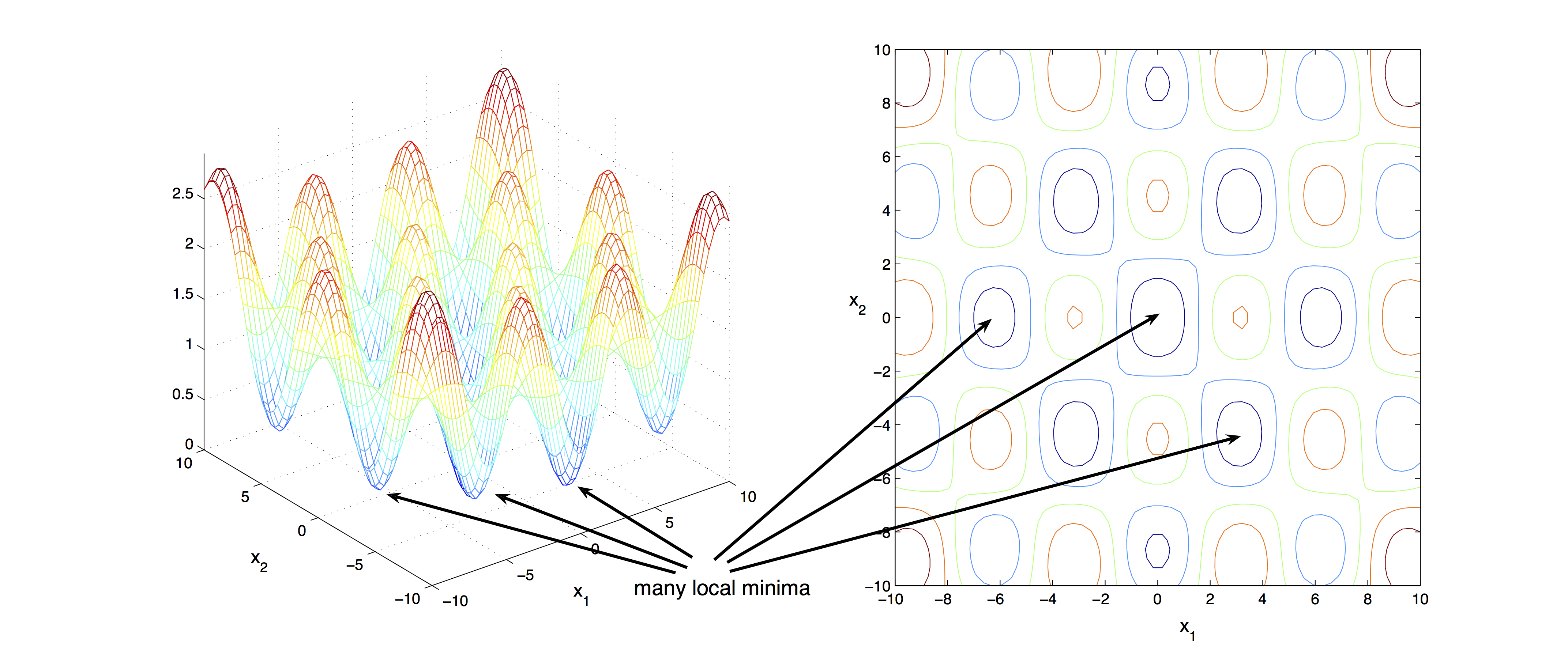
This is all we like to cover about constrained nonlinear optimization. In the subsequent part of this lecture, we shall only review the basics on convexity and unconstrained optimization. Before we proceed to the solution algorithms, it is important to note that whenever we call a point an optimal solution, we almost always refer to a local stationary point. The following figure shows that even a two dimensional unconstrained optimization problem may involve many local minima. Global optimization problems are in general very difficult and beyond the scope of this lecture.

 Convexity

In nonlinear optimization the concept of convexity plays a very important role. We have convex sets and convex functions.

A set $\CS\in\RR^n$ is convex if the straight line segment connecting any two points in $\CS$ lies entirely inside $\CS$. Formally, for any two points $x, y \in \CS$, we have

$$ \alpha x + (1 - \alpha)y \in \CS, \hspace{5mm} \mbox{for all } \alpha \in [0,1]. $$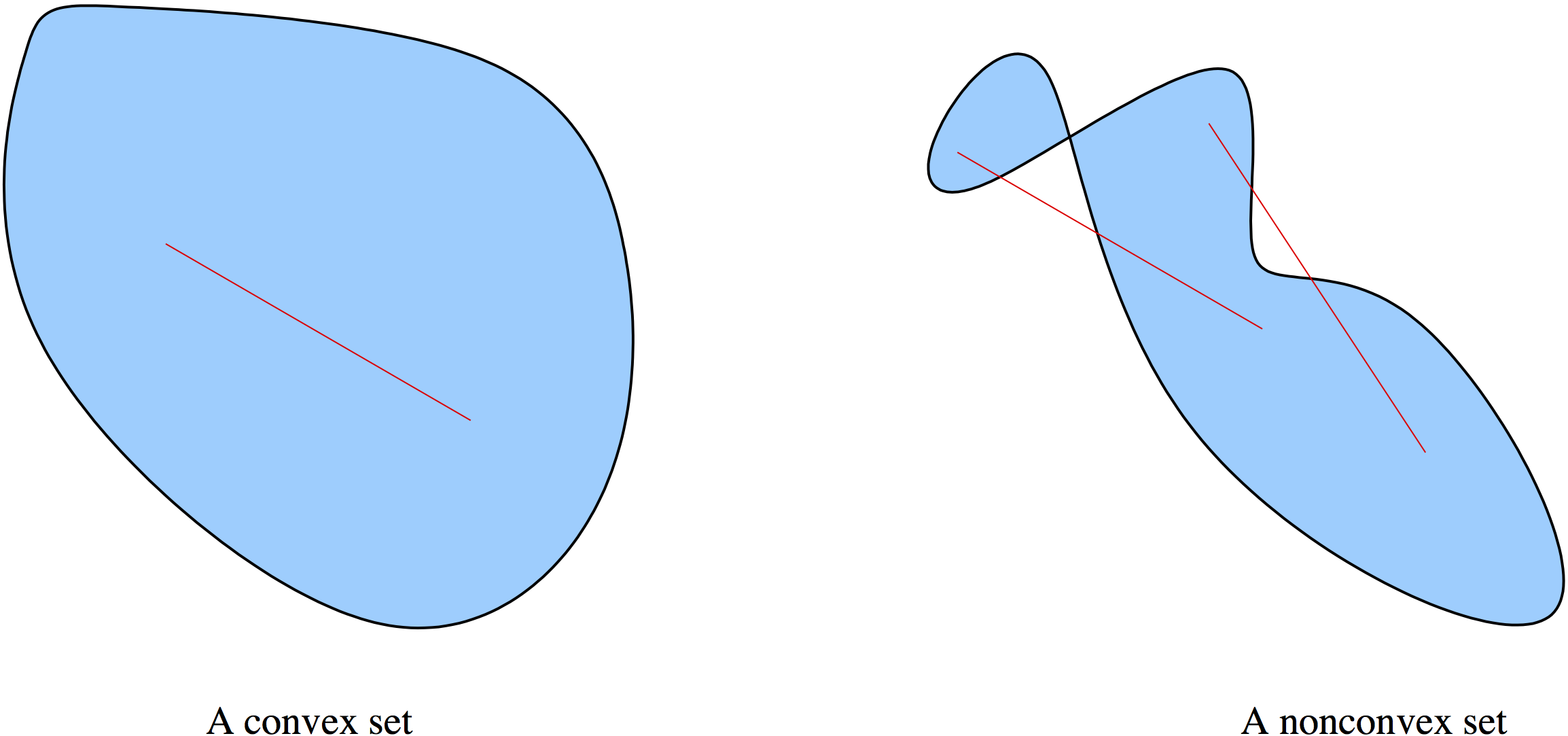

A function $f$ is convex, if its domain is a convex set and if for any two points $x$ and $y$ in this domain, the graph of $f$ lies below the line segment connecting the points $(x, f (x))$ and $(y, f (y))$. Formally,

$$ f(\alpha x + (1 - \alpha)y) \leq \alpha f(x) + (1 - \alpha)f(y), \hspace{5mm} \mbox{for all } \alpha \in [0,1]. $$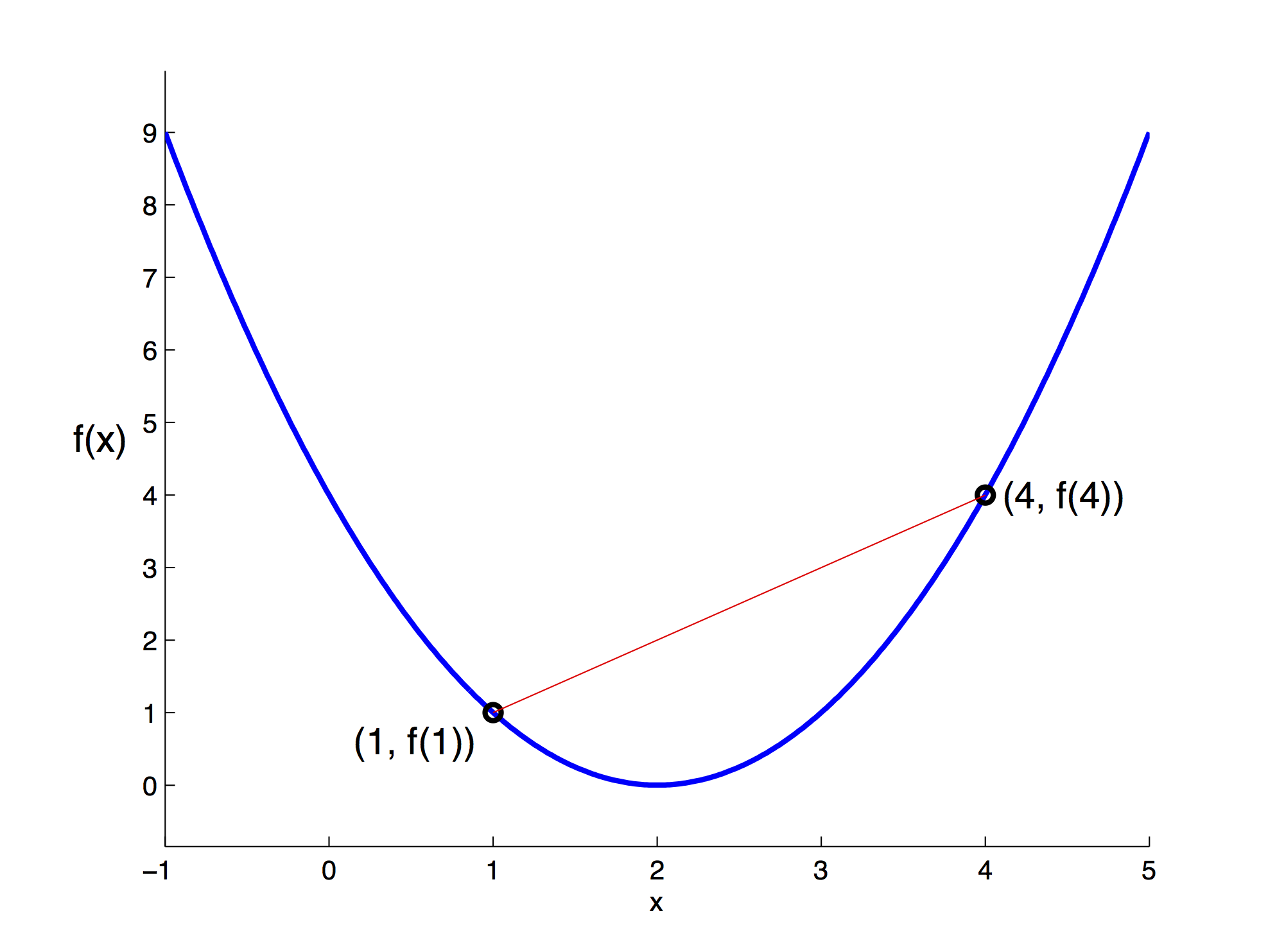

A function $f$ is concave, if $−f$ is convex. Convex functions play an important role in optimization for various reasons. For instance:

• When dealing with unconstrained optimization, the local minimizer is also a global minimizer.
• Less-than-or-equal to constraints formed with convex functions yield convex sets.
• Roughly speaking, in many cases working with convex functions guarantee that the necessary conditions are also sufficient.
• Convex functions are also used for locally approximating difficult nonconvex functions.

 Unconstrained Optimization

We consider the following problem:

$$ \begin{array}{ll} \minimize & f(x) \\ \subto & x \in \RR^n. \end{array} $$

When the objective function $f$ is smooth, even better twice continuously differentiable, we can discuss the necessary and sufficient conditions for a point $x^* \in \RR^n$ to be a local minimizer. These conditions can be easily proved by using the Taylor’s theorem from elementary calculus.

Taylor's Theorem: Let $f:\RR^n \ra \RR$ be continuously differentiable and $p \in \RR^n$. Then, $$ f(x+p) = f(x) + \df(x + tp)\tr p \hspace{5mm} \mbox{for some } t \in (0,1). $$ If $f$ is twice continuously differentiable, then $$ \df(x+p) = \df(x) + \int_0^1 \ddf(x + tp)p dt $$ and $$ f(x+p) = f(x) + \df(x)\tr p + \frac{1}{2} p\tr \ddf(x + tp)p \hspace{5mm} \mbox{for some } t \in (0,1). $$ Equivalently, we have $$ f(x+p) = f(x) + \df(x)\tr p + \frac{1}{2} p\tr \ddf(x)p + o(\|p\|^2). $$

Now we are ready to compile the conditions for optimality.

First Order Necessary Conditions: Let $x^* \in \RR^n$ be a local minimizer and $\df$ be continuous in an open neighborhood of $x^*$. Then $\df(x^*) = 0$.

A point $x^*$ satisfying $\df(x^*)=0$ is called a stationary point and a matrix $A$ is called positive semidefinite, if $p\tr A p \geq 0$ for all $p \in \RR^n$. Likewise, the matrix is called positive definite, if $p\tr A p > 0$ for all $p \in \RR^n$ with $p \neq 0$.

Second Order Necessary Conditions: Let $x^* \in \RR^n$ be a local minimizer and $\ddf$ be continuous in an open neighborhood of $x^*$. Then $\df(x^*) = 0$ and $\ddf(x^*)$ is positive semidefinite.

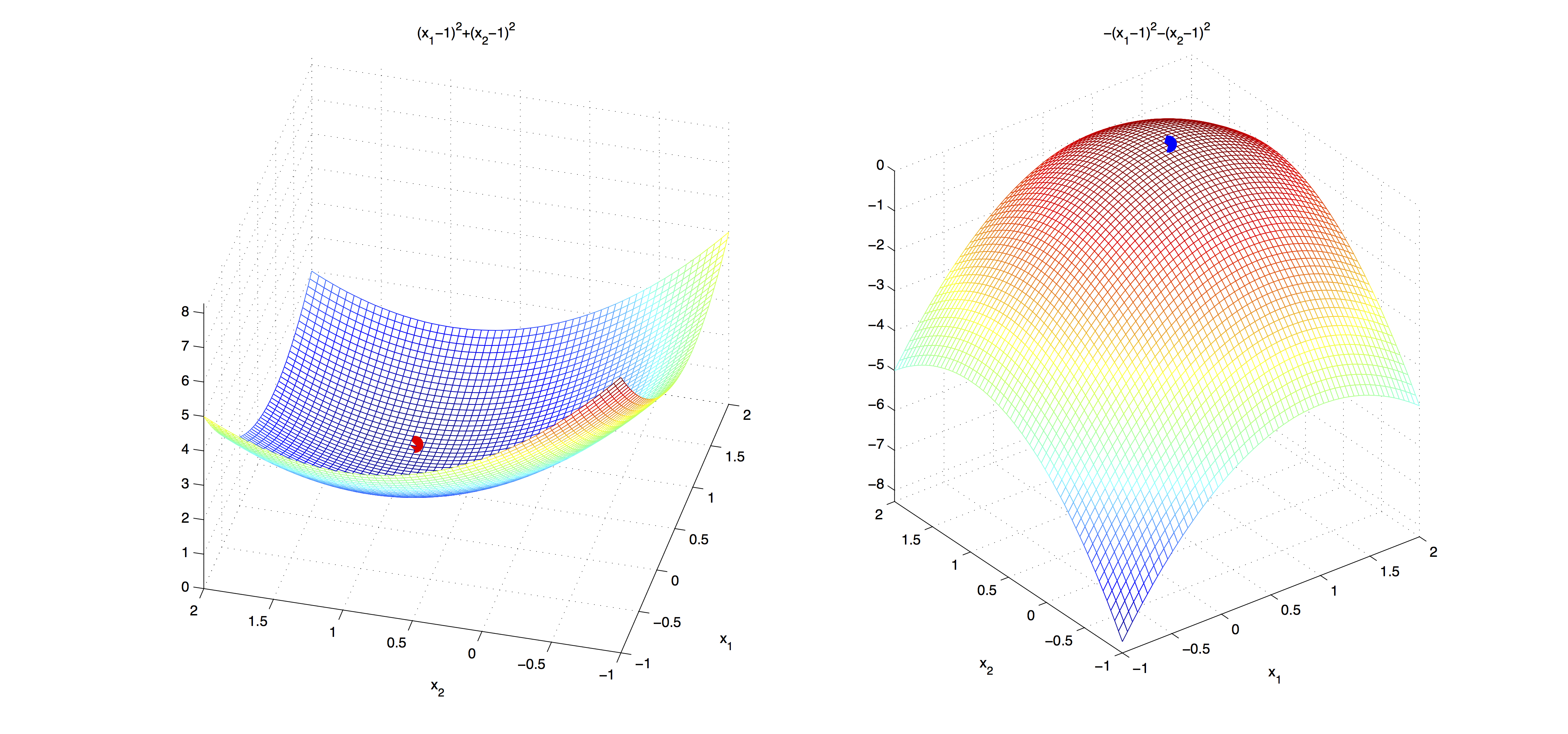
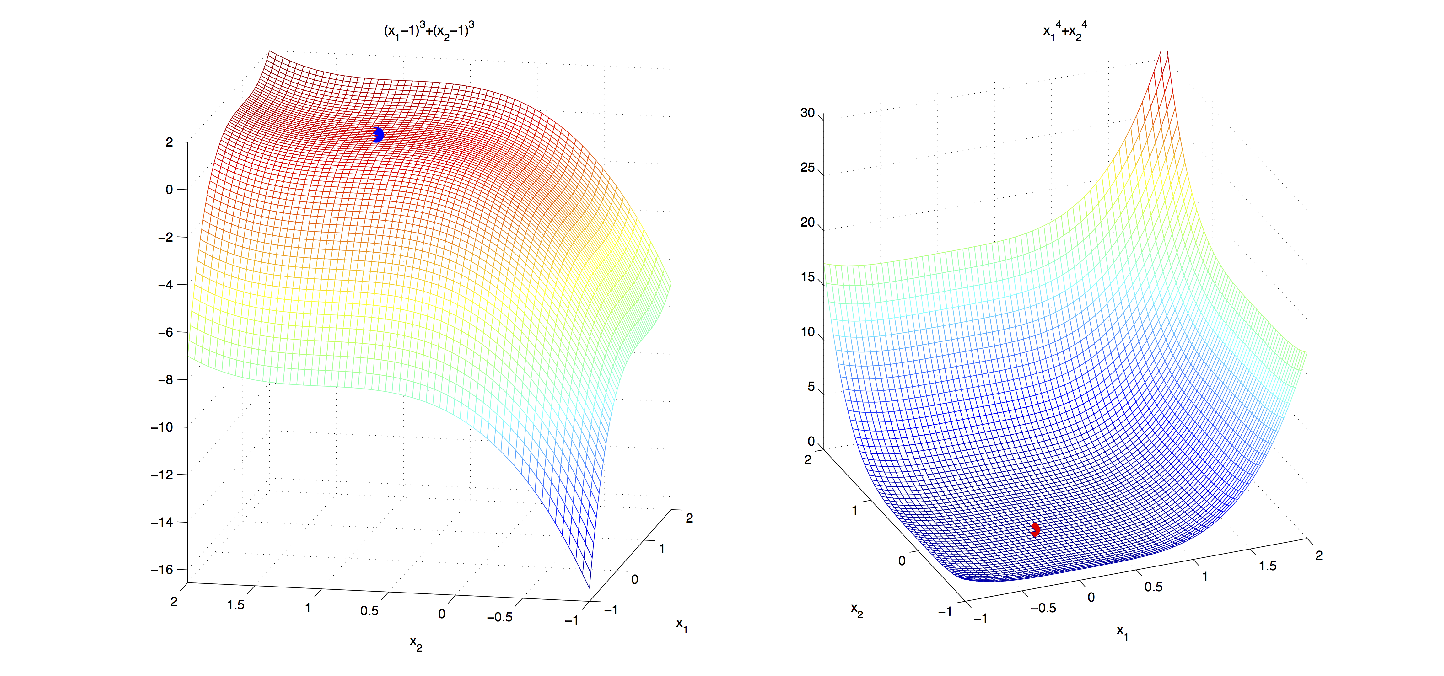
In the figure below, the first order necessary conditions are satisfied for both functions. However, the second order necessary conditions are satisfied only by the function on the left.

Second Order Sufficient Conditions: Let $\ddf$ be continuous in an open neighborhood of $x^* \in \RR^n$, $\ddf(x^*)$ be positive definite and $\df(x^*) = 0$. Then $x^*$ is a strict local minimizer of $f$.

The following figure demonstrates a case, where second order necessary conditions are not enough to identify a local minimum.

Note that the second order sufficient conditions immediately show that if $f$ is a convex differentiable function, then any stationary point of $f$ is a global minimizer.

Almost all unconstrained optimization algorithms generate a sequence of iterates, $x_k$, where the initial point $x_0$ is usually provided by the user. It is important to note that in the subsequent part of these notes, the iterates will be shown by subscripts. Do not confuse them with the components of the vector $x$ as we have used before.

There are two fundamental appraoches in unconstrained optimization. These are line search methods and trust region methods.

In line search methods, first a direction $p_k$ is chosen at iteration $k$ and then, the algorithm searches along this direction to select a favorable step length $\alpha_k$. One option is to solve the one-dimensional optimization problem:

$$ \alpha_k = \underset{\alpha > 0}{\arg\min} \ f(x_k + \alpha p_k). $$

This could be too much to ask. Therefore, many algorithms are content with an approximate but acceptable step length. To give an example, we next use line search method to find the minimum of the well-known Rosenbrock function

$$ f(y, z) = 100*(z - y^2)^2 + (1 - y)^2. $$

fun = @(x)100*(x(2) - x(1)^2)^2 + (1 - x(1))^2;
dfun = @(x)[-400*x(1)*(x(2) - x(1)^2) - 2*(1 - x(1)); 200*(x(2) - x(1)^2)];
x = [0.8; -8]; maxiter = 500; fhist = zeros(1, maxiter);
iter = 1;
while (iter < maxiter)
    p = -dfun(x);
    if (norm(p) < 1.0e-4)
        break;
    end
    [alpha, fhist(iter)] = fminbnd(@(alpha)fun(x + alpha*p), 0, 1);
    x = x + alpha*p;
    iter = iter + 1;
end
fprintf('Solution at iteration %d: (%f, %f)\nNorm of gradient: %f', ...
    iter, x(1), x(2), norm(p));
% Plot of first 10 iterations
plot(1:10, fhist(1:10), 'b-', 'LineWidth', 3); 
axis([1,10]); grid on;
xlabel('Iterations');
ylabel('Objective Function Value');

Solution at iteration 500: (1.495739, 2.238607)
Norm of gradient: 1.342154

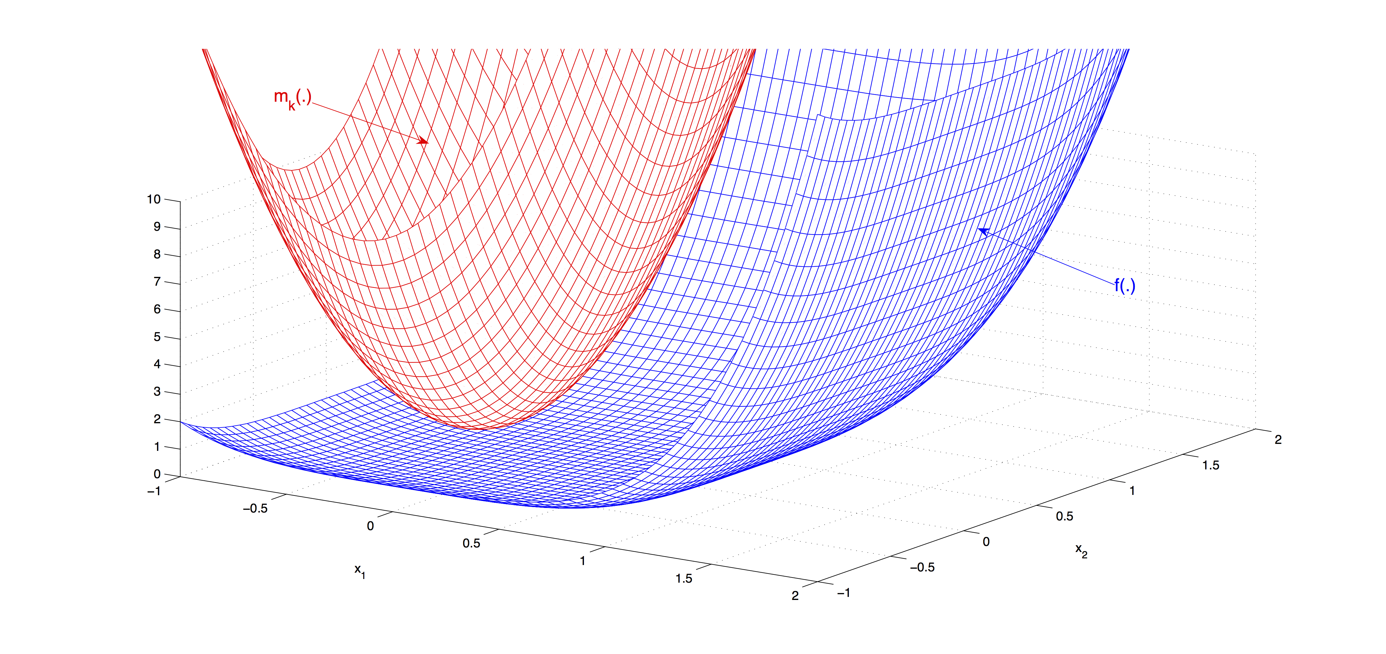
In trust region methods, the core idea is to construct at iteration $k$, a model function $m_k$, which locally approximates the original function $f$ around $x_k$. Since the model function is just a local approximation, the model may not be trustworthy if a large step is taken. Therefore, the model function is optimized over a trust region that basically defines all possible steps with acceptable lengths. That is, at every iteration one needs to solve

$$ \underset{p}{\min} \left\{m_k(x_k + p) : x_k + p \mbox{ lies inside the trust region}\right\}. $$

A typical region is defined by the Euclidean ball $\{p : \|p\| \leq \Delta\}$ with radius $\Delta > 0$. If the solution to the model function does not reflect an acceptable reduction in $f$, then the trust region radius is decreased. When the successive reductions in $f$ are good, then the trust region radius is increased. In most cases, $m_k(\cdot)$ is a quadratic function defined as

$$ m_k(x_k + p) = f(x_k) + p\tr\df(x_k) + \frac{1}{2} p\tr B_k p, $$

where matrix $B_k$ is usually the Hessian $\ddf(x_k)$ or its approximation at iteration $k$. An example function $f$ and its local approximation $m_k$ are shown in the next figure.

When we compare line search and trust region strategies, there are several important points worth mentioning:

1. In the trust region strategy, each time the trust region is shrinked, the optimal direction $p$ may change. In case of line search, the direction remains the same.
2. In line search strategy we seek for an acceptable step length along the given direction. In case of trust region, the direction and the step are determined at the same time.
3. In line search methods, the step length is determined by solving a one-dimensional optimization problem. On the other hand, in trust region methods a quadratic $n$-dimensional optimization problem needs to be solved.
4. The choice of $p_k$ in line search strategy and the choice of $B_k$ in trust region strategy are very crucial. In fact, these two choices are closely related.

Clearly, any direction can not be acceptable. So what kind of directions are we interested in? Using Taylor's theorem we have

$$ f(x_k + \alpha p) = f(x_k) + \alpha \underset{<0}{\underbrace{p\tr\df(x_k)}} + O(\alpha^2). $$

This shows that the angle $\theta$ between $p$ and $-\df(x_k)$ better be strictly less than $\pi/2$, since

$$ p\tr\df(x_k) = \|p\|\|\df(x_k)\|\cos\theta < 0. $$

Such a direction $p$ is called a descent direction and a sufficiently small step length along a descent direction guarantees a decrease in the objective function value. Naturally, it is desirable to find the descent direction $p$, which yields the largest decrease. This particular direction is the solution to the problem

$$ \underset{p}{\min} \{ p\tr\df(x_k) : \|p\|=1\}. $$

Using now the relation $p\tr\df(x_k) < 0$, the optimal solution to the above problem is

$$ p=\frac{-\df(x_k)}{\|\df(x_k)\|}. $$

The infamous steepest descent method uses $p_k = -\df(x_k)$ as the descent direction. A very important seach direction is the Newton direction. The main idea is to provide a quadratic approximation to the objective function

$$ f(x_k + p) \approx f(x_k) + p\tr\df(x_k) + \frac{1}{2} p\tr\ddf(x_k)p := m_k(p). $$

The minimum of the approximate function $m_k(p)$ can be found by setting the derivative equal to zero. If we assume that $\ddf(x_k)$ is invertible, then the optimal direction is given by

$$ p_k^{N} = -{\ddf(x_k)}\inv\df(x_k). $$

Notice that $p_k^N$ qualifies as a descent direction if $\ddf(x_k)$ is positive definite, since

$$ \df(x_k)\tr p_k^{N}=-p_k^{N}\ddf(x_k)p_k^{N} \leq -\sigma_k \|p_k^{N}\|^2 $$

for some $\sigma_k > 0$. Unless the gradient $\df(x_k)$ is zero (so is $p_k^{N}$), we have $\df(x_k)\tr p_k^{N} < 0$.

There are two issues with the Newton direction: (i) $\ddf(x_k)$ may not be invertible, then $p_k^{N}$ is undefined. (ii) $\ddf(x_k)$ may not be positive definite, then $p_k^{N}$ may not be a descent direction. (This can be overcome by some modifications.)

The major disadvantage of using Newton direction is to compute the Hessian $\ddf(\cdot)$ at every iteration. Quasi-Newton methods, on the other hand, try to avoid computing the Hessian at every iteration. Instead, they use a Hessian approximation $B_k$, which is updated according to the new information gained from the gradients as iterations progress. Even better, the inverse matrix $B\inv_{k+1}$ of iteration $k+1$ is computed very fast by using the inverse matrix of previous iteration, $B\inv_{k}$.

Next we solve the Rosenbrock function again. This time we use both the steepest descent and the quasi-Newton methods. The plot shows that the quasi-Newton method converges much faster than the steepest descent method.

% SD Method
fun = @(x)100*(x(2) - x(1)^2)^2 + (1 - x(1))^2;
dfun = @(x)[-400*x(1)*(x(2) - x(1)^2) - 2*(1 - x(1)); 200*(x(2) - x(1)^2)];
x0 = [0.8; -8]; maxiter = 500; sd_fhist = zeros(1, maxiter);
iter = 1; x=x0;
while (iter < maxiter)
    p = -dfun(x);
    if (norm(p) < 1.0e-4)
        break;
    end
    [alpha, sd_fhist(iter)] = fminbnd(@(alpha)fun(x + alpha*p), 0, 1);
    x = x + alpha*p;
    iter = iter + 1;
end
fprintf('SD Solution at iteration %d: (%f, %f)\nNorm of gradient: %f\n', ...
    iter, x(1), x(2), norm(p));

% QN Method
x=x0;
qn_fhist = zeros(1, maxiter);
I = eye(length(x0));  df = dfun(x);
iter = 1; Binv = I;
while (iter < maxiter)
    p = -Binv*df;
    if (norm(p) < 1.0e-4)
        break;
    end
    [alpha, qn_fhist(iter)] = fminbnd(@(alpha)fun(x + alpha*p), 0, 1);
    x = x + alpha*p;
    s = alpha*p;
    yold = df;
    df = dfun(x);
    y = df - yold;
    if (abs(y'*s) <= 1.0e-4^2) 
        Binv = I;
    else
        Binv = (I - (s*y')/(y'*s))*Binv*(I - (y*s')/(y'*s)) + (s*s')/(y'*s); 
    end 
    iter = iter + 1;
end
fprintf('QN Solution at iteration %d: (%f, %f)\nNorm of gradient: %f', ...
    iter, x(1), x(2), norm(p));
plot(1:10, sd_fhist(1:10), 'b-', 'LineWidth', 3); hold on;
plot(1:10, qn_fhist(1:10), 'r-', 'LineWidth', 3); hold off;
legend('SD', 'QN'); axis([1,10]); grid on;
xlabel('Iterations');
ylabel('Objective Function Value');

SD Solution at iteration 500: (1.495739, 2.238607)
Norm of gradient: 1.342154
QN Solution at iteration 85: (1.000002, 1.000003)
Norm of gradient: 0.000004

In fact, line search and trust region strategies are quite related. Suppose that $B_k = 0$ in the objective function of the trust region subproblem, then we obtain

$$ \underset{p}{\min}\left\{ f(x_k) + p\tr\df(x_k) : \|p\|_2 \leq \Delta_k \right\}. $$

Notice that the optimal solution to this problem is

$$ p_k = -\Delta_k \frac{\df(x_k)}{\|\df(x_k)\|}, $$

which is the steepest descent direction with step length $\Delta_k$.

A very successful implementation of trust region methods uses $B_k=\ddf(x_k)$ (trust-region Newton method). An important point here is that the trust-region problem always has a solution $p_k$. That is $B_k$ does not have to be positive definite. Whenever, $B_k$ is given as a quasi-Newton approximation, the resulting implementation becomes trust region quasi-Newton method.

---

References

1. Nocedal, J. and S. J. Wright (2006). Numerical Optimization, 2nd Edition, New York:Springer.
2. Birbil, Ş. İ. (2015). IE 509 Class Notes, Sabancı University.