$ \newcommand{\CF}{\mathcal{F}} \newcommand{\CI}{\mathcal{I}} \newcommand{\CJ}{\mathcal{J}} \newcommand{\CL}{\mathcal{L}} \newcommand{\CX}{\mathcal{X}} \newcommand{\CP}{\mathcal{P}} \newcommand{\CR}{\mathcal{R}} \newcommand{\RR}{\mathbb{R}} \newcommand{\NN}{\mathbb{N}} \newcommand{\ZZ}{\mathbb{Z}} \newcommand{\ra}{\rightarrow} \newcommand{\la}{\leftarrow} \newcommand{\inv}{^{-1}} \newcommand{\maximize}{\mbox{maximize }} \newcommand{\minimize}{\mbox{minimize }} \newcommand{\subto}{\mbox{subject to }} \newcommand{\tr}{^{\intercal}} $
Dantzig-Wolfe Decomposition and Column Generation
In this lecture, we shall essentially talk about rewriting a set of constraints in terms of the extreme points and the extreme directions of the polyhedron formed with those constraints. Although this approach leads to a problem with less number of constraints, the number of variables increases exponentially. To deal with a problem involving a large number of columns, we shall discuss a method that selects the most promising columns in an iterative manner.
Dantzig-Wolfe Decomposition
Here is the linear programming (LP) problem that we shall use throughout this section:
$$ \tag{P} \begin{array}{rcll} Z_P & = & \maximize & c\tr x \\ & & \subto & Ax \leq b, \\ & & & Dx \leq d, \\ & & & x \geq 0, \end{array} $$where $A$ is $m \times n$ and $D$ is $k \times n$. Let us now define the polyhedron $\CX$ given by
$$ \CX = \{x \in \RR^n : Dx \leq d, \ x \geq 0\}. $$As we have covered in Lecture 2, we can obtain the Lagrangian dual problem
$$ Z_L = \min\{ Z_L(\lambda) : \lambda \geq 0\}, $$where $\lambda \in \RR^m$ is the multiplier vector and
$$ Z_L(\lambda) = \max\{ c\tr x + \lambda\tr(b - Ax) : x \in \CX \}. $$Suppose for now that $\CX$ is bounded, and hence, it can be represented by its extreme points only (Minkowski's Represantaion Theorem; see appendix). Let $\CP_\CX = \{x^p, p \in \CI_\CP\}$ denote the set of extreme points of $\CX$. Then, we have $$ Z_L(\lambda) = \max\{ c\tr x^p + \lambda\tr(b - Ax^p) : x^p \in \CP_\CX \} = \max_{p \in \CI_\CP} \{c\tr x^p + \lambda\tr(b - Ax^p)\}. $$
Thus, the Lagrangian dual problem can be equivalently written as
$$ \tag{L} \begin{array}{rcllr} Z_L & = & \minimize & z & \\ & & \subto & z \geq c\tr x^p + \lambda\tr(b - Ax^p), \ p \in \CI_\CP & (\mu_p)\\ & & & \lambda \geq 0. \end{array} $$Clearly, this problem has a huge number of constraints. Let $\mu_p$, $p \in \CI_\CP$ be the dual variables corresponding to the the first set of constraints above, then the dual of this problem becomes
$$ \begin{array}{crl} \maximize & \sum_{p \in \CI_\CP} (c\tr x^p)\mu_p \\ \subto & \sum_{p \in \CI_\CP} \mu_p = 1, \\ & \sum_{p \in \CI_\CP} (b - Ax^p)\mu_p \geq 0, \\ & \mu_p \geq 0, p \in \CI_\CP. \end{array} $$After organizing the terms of the problem, we obtain
$$ \tag{MP} \begin{array}{rcll} Z_{MP} & = & \maximize & c\tr (\sum_{p \in \CI_\CP} \mu_p x^p) \\ & & \subto & A(\sum_{p \in \CI_\CP} \mu_p x^p) \leq b, \\ & & & \sum_{p \in \CI_\CP} \mu_p = 1,\\ & & & \mu_p \geq 0, p \in \CI_\CP. \end{array} $$This problem is known as the master problem in Dantzig-Wolfe decomposition. Observe that the polyhedron $\CX$ is represented in terms of its extreme points. Thus, using Minkowski's representation theorem, problem (MP) is simply equivalent to problem (P). Therefore $Z_{MP} = Z_P$.
The master problem involves a very large number of variables as we require a column for every extreme point of $\CX$. Instead of generating all columns at the outset, one idea is to start with only $t$ columns and solve
$$ \tag{RMP} \begin{array}{rcll} Z_{RMP} & = & \maximize & c\tr (\sum_{p=1}^{t} \mu_p x^p) \\ & & \subto & A(\sum_{p=1}^{t} \mu_p x^p) \leq b, \\ & & & \sum_{p=1}^{t} \mu_p = 1,\\ & & & \mu_p \geq 0, p = 1, \dots, t. \end{array} $$This problem is called the restricted master problem. Any solution to (RMP) is a feasible solution for (MP). If we can observe that all those remaining columns indexed by $\CI_\CP \backslash \{1, \dots, t\}$ have nonpositive reduced cost, then the current optimal solution of (RMP) is also optimal for (MP). However, if there are columns with positive reduced costs, then we introduce those columns to (RMP) and form the next (RMP) with more columns. This procedure is also known as column generation and we shall cover it in the next subsection.
As a last point of this section, it is relatively easy to see that solving (MP) with column generation method is equivalent to applying a cutting plane method to the Lagrangian dual problem (L). This is not surprising as we have formed (MP) by taking the dual of (L).
Column Generation
Consider the LP problem in standard form:
$$ \begin{array}{ll} \minimize & c\tr x \\ \subto & Ax =b, \\ & x \geq 0, \end{array} $$where $A$ is an $m \times n$ matrix. Recall from Lecture 1 that the reduced cost of a nonbasic variable $x_k$ is given by
$$ \bar{c}_k = (c\tr_N - \underset{\mbox{dual optimal}}{\underbrace{c\tr_B B^{-1}}}N)_k, $$where $B$ is the basis matrix and the remaining columns of $A$ constitute the matrix $N$. If we now denote the columns of $A$ by $a_1, a_2, \dots, a_m$, then we can simply write
$$ \bar{c}_k = c_k - c\tr_B B^{-1}a_k. $$Suppose $x_s$ is the nonbasic variable with the minimum reduced cost. That is,
$$ \bar{c}_s = \min_k\{c_k - c\tr_B B^{-1}a_k\}. $$There are two possible cases that can occur in the Simplex method:
- The reduced cost of all nonbasic variables are nonnegative; i.e. $\bar{c}_s \geq 0$. Then, the current basis is optimal.
- The reduced cost of at least one nonbasic variable is negative; i.e. $\bar{c}_s < 0$. Then, the current basis is not optimal and $x_s$ or some other variable with a negative reduced cost enters the basis and we carry on with the Simplex iterations.
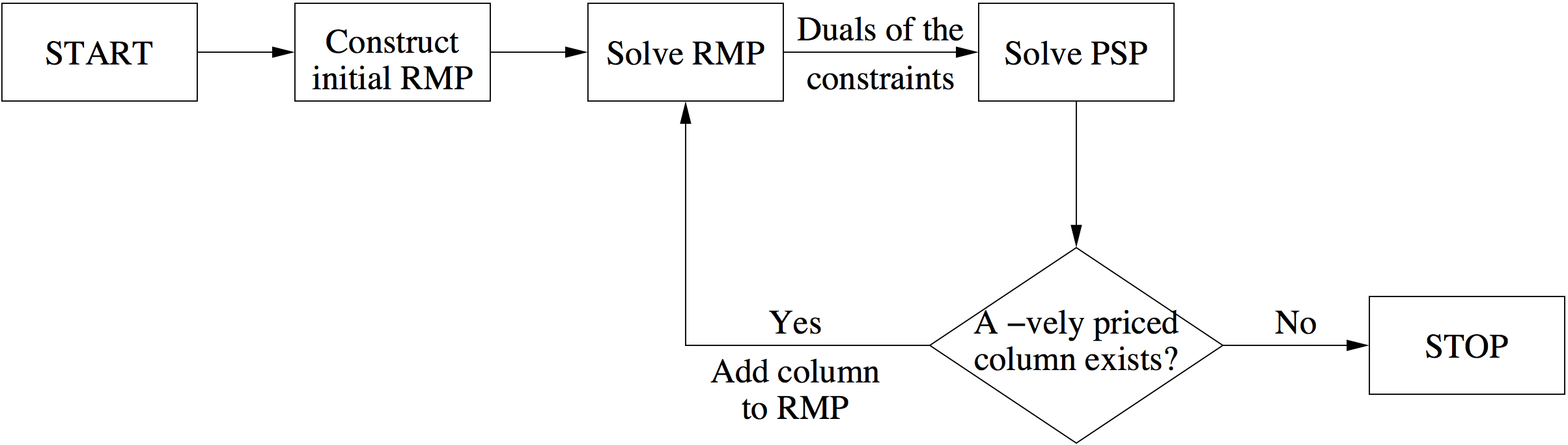
This algorithm is known as column generation. We remark that for large-scale problems, where the number of variables ($n$) is far more than the number of constraints ($m$), finding $x_s$ or some other variable with a negative reduced cost usually requires solving a separate problem, known as pricing subproblem (PSP). The following flowchart illustrates the steps of column generation when a separate PSP is present.
A famous example is the cutting stock problem, where the PSPs boil down to integer knapsack problems.
Example
Suppose a company produces three sizes (2 meters, 5 meters and 7 meters) of iron bars used in construction business. These sizes are cut from 26-meter stock bars. The customer demands for 2-meter, 5-meter and 7-meter bars are 32, 28 and 16, respectively. The objective is to minimize the number of stock bars such that the customer demand is met.
Each stock bar can be cut according to a combination. For instance, from a stock bar one can cut 4 times 2-meter bars, 2 times 5-meter bars and one time a 7-meter bar. Clearly, there are many other possible combinations.
Let $x_i$ denote the number of stock bars cut according to combination $i$. Then, our mathematical programming model becomes
$$ \begin{array}{ll} \minimize & \sum_{i=1}^n x_i \\ \subto & \sum_{i=1}^n a_{i(2)} x_i \geq 32, \\ & \sum_{i=1}^n a_{i(5)} x_i \geq 28, \\ & \sum_{i=1}^n a_{i(7)} x_i \geq 16, \\ & x_i \geq 0 \mbox{ and integer}, \end{array} $$where $a_{i(2)}$, $a_{i(5)}$, $a_{i(7)}$ show the number of times 2-meter, 5-meter and 7-meter bars occur in combination $i$, respectively. This is an integer programming problem but we shall focus on solving its LP relaxation.
Note that a combination must satisy
$$ 2 a_{i(2)} + 5 a_{i(5)} + 7 a_{i(7)} \leq 26. $$Of course, the trivial combinations corresponding to unit vectors satisfy the above inequality. These combinations create a lot of waste but we can just start our column generation method with them.
A = eye(3);
n = length(A);
b = [32; 28; 16];
c = ones(n, 1);

lb = zeros(n, 1); ub = [];
ctype = repmat("L", 1, 3); vartype = repmat("C", 1, n);
[x, fval, ~, extra] = glpk(c, A, b, lb, ub, ctype, vartype, 1);
fprintf('Optimal objective function value: %f\n', fval);
fprintf('Optimal solution: '); disp(x');
fprintf('Dual optimal solution: '); extra.lambda'
Suppose our next combination is $(4, 2, 1)\tr$. Let's check its reduced cost.
ck = 1;
ak = [4; 2; 1];
cBBinv = extra.lambda';
ckbar = ck - cBBinv*ak
Its reduced cost is negative. So we can add it to our problem.
A = [A, ak];
n = length(A);
b = [32; 28; 16];
c = ones(n, 1);

lb = zeros(n, 1); ub = [];
ctype = repmat("L", 1, 3); vartype = repmat("C", 1, n);
[x, fval, ~, extra] = glpk(c, A, b, lb, ub, ctype, vartype, 1);
fprintf('Optimal objective function value: %f\n', fval);
fprintf('Optimal solution: '); disp(x');
Adding this new combination reduced the objective function from 76 to 16. This is nice. However, so far we have been providing the combinations. The next task is to model a problem so that the combination with the minimum reduced cost is generated after solving this PSP subproblem. Here it is:
$$ \begin{array}{ll} \minimize & 1 - c_B\tr B^{-1}a_k \\ \subto & 2 a_{k(2)} + 5 a_{k(5)} + 7 a_{k(7)} \leq 26, \\ & a_{k(2)}, a_{k(5)}, a_{k(7)} \geq 0 \mbox{ and integer.} \end{array} $$This is a knapsack problem that we can solve with specialized algorithms like dynamic programming. For our lecture, we shall just solve this integer programming problem with CPLEX.
D = [2, 5, 7];
d = -extra.lambda';
e = 26;
lbks = zeros(3, 1); ubks = [];
ctypeks = "U"; vartypeks = repmat("I", 1, 3);
[ak, barcs] = glpk(d, D, e, lbks, ubks, ctypeks, vartypeks, 1);
fprintf('New combination is: '); disp(ak');
fprintf('Its reduced cost: %f', barcs+1);
We have a new combination with a negative reduced cost. So we add column $(0, 0, 3\tr)$ and continue. Here is the entire script that solves the cutting stock problem.
A = eye(3); b = [32; 28; 16];
D = [2, 5, 7]; e = 26;
n = length(A);
c = ones(n, 1);

lb = zeros(n, 1); ub = [];
ctype = repmat("L", 1, 3); vartype = repmat("C", 1, n);
lbks = zeros(3, 1); ubks = [];
ctypeks = "U"; vartypeks = repmat("I", 1, 3);

barcs = -100; tol = -0.001;
while (barcs+1 < tol)
    [xopt, fval, ~, extra] = glpk(c, A, b, lb, ub, ctype, vartype, 1);
    fprintf('Optimal objective function value: %f\n', fval);
    d = -extra.lambda';
    [ak, barcs] = glpk(d, D, e, lbks, ubks, ctypeks, vartypeks, 1);
    fprintf('New column''s reduced cost: %f\n', barcs+1);
    if (barcs+1 < tol)
        A = [A, ak];
        n = length(A); c = ones(n, 1);
        vartype = repmat("C", 1, n);
        lb = zeros(n, 1);
    end
end
fprintf('\nOptimal solution: '); disp(xopt(xopt>0)');
fprintf('Selected combinations: \n'); disp(A(:, xopt>0));
Column Generation Applied to Dantzig-Wolfe Decomposition
Consider a LP problem of the form
$$ \tag{LP-Base} \begin{array}{rcll} z^* & = & \minimize & c\tr x \\ &&\subto & Ax =b, \\ && & Dx = d, \\ && & x \geq 0, \end{array} $$where $A$ is $m \times n$ and $D$ is $k \times n$. Suppose that we rewrite the first set of constraints in terms of its extreme points and extreme directions. Thus, for the polyhedron
$$ \CX = \{x \in \RR^n : Dx = d, \ x \geq 0\}, $$we define the set of extreme points and the set of extreme directions as $\CP_\CX = \{x^p, p \in \CI_\CP\}$ and $\CR_\CX = \{x^r, r \in \CI_\CR\}$, respectively. Using again the representation theorem, we can rewrite problem (LP-Base) and obtain the master problem
$$ \tag{LP-MP} \begin{array}{rcllr} z^*&=&\minimize & \sum_{p \in \CI_\CP}\mu_p(c\tr x^p) + \sum_{r \in \CI_\CR}\nu_r(c\tr x^r) &\\ &&\subto & \sum_{p \in \CI_\CP} \mu_p(Ax^p) + \sum_{r \in \CI_\CR} \nu_r(Ax^r) = b, & (\pi)\\ && & \sum_{p \in \CI_\CP} \mu_p = 1, & (\alpha)\\ && & \mu_p \geq 0, p \in \CI_\CP, & \\ && & \nu_r \geq 0, r \in \CI_\CR.& \end{array} $$This problem has $k-1$ less constraints than (LP-Base). However, the number of variables is extremely large. We denote the dual variables associated with the first set of constraints and the next constraint with $\pi$ and $\alpha$, respectively. Then, we can write the dual problem
$$ \tag{LP-DMP} \begin{array}{rcll} z^*&=&\maximize & b\tr \pi + \alpha\\ &&\subto & (Ax^p)\tr \pi + \alpha \leq c\tr x^p, p \in \CI_\CP,\\ && & (Ax^r)\tr \pi \leq c\tr x^r, r \in \CI_\CR. \end{array} $$Note that the reduced cost of $x^p$, $p \in \CI_\CP$ is
$$ c\tr x^p - (Ax^p)\tr \pi - \alpha = (c - A\tr\pi)\tr x^p - \alpha. $$Likewise, the reduced cost of $x^r$, $r \in \CI_\CR$ is
$$ c\tr x^r - (Ax^r)\tr \pi = (c - A\tr\pi)\tr x^r. $$Now, we can discuss how to solve (LP-MP) with column generation. Suppose at a given iteration, we have a subset of columns (LP-MP) indexed by $\bar{\CI}_\CP \subseteq \CI_\CP$ and $\bar{\CI}_\CR \subseteq \CI_\CR$. Then, the restricted master problem simply becomes
$$ \tag{LP-RMP} \begin{array}{rcll} \bar{z} &=&\minimize & \sum_{p \in \bar{\CI}_\CP}\mu_p(c\tr x^p) + \sum_{r \in \bar{\CI_\CR}}\nu_r(c\tr x^r)\\ &&\subto & \sum_{p \in \bar{\CI}_\CP} \mu_p(Ax^p) + \sum_{r \in \bar{\CI}_\CR} \nu_r(Ax^r) = b, \\ && & \sum_{p \in \bar{\CI}_\CP} \mu_p = 1,\\ && & \mu_p \geq 0, p \in \bar{\CI}_\CP,\\ && & \nu_r \geq 0, r \in \bar{\CI}_\CR. \end{array} $$Clearly, $\bar{z} \geq z^*$. If we denote the optimal dual solution of this LP by $(\bar{\pi}, \bar{\alpha})$, then our PSP for column generation simply becomes
$$ \bar{c}_s = \min_{x \in \CX} \ (c - A\tr\bar{\pi})\tr x \ \ - \overset{constant}{\overbrace{\bar{\alpha}}} $$We solve this LP problem. There are three possible outcomes of this subproblem:
- $\bar{c}_s < 0$ and the subproblem has a finite objective function value. Then, we have an extreme point, $\bar{x}^p$, $p \in \CI_\CP \backslash \bar{\CI}_\CP$ that will be added to (LP-RMP) as a new column $$ \left[ \begin{array}{c} c\tr\bar{x}^p \\ A\bar{x}^p \\ 1 \end{array} \right] $$ and the index set is updated, $\bar{\CI}_\CP \leftarrow \bar{\CI}_\CP \cup \{p\}$.
- $\bar{c}_s < 0$ and the subproblem is unbounded. Then, we have an extreme recession direction, $\bar{x}^r$, $r \in \CI_\CR \backslash \bar{\CI}_\CR$ that will be added to (LP-RMP) as a new column $$ \left[ \begin{array}{c} c\tr\bar{x}^r \\ A\bar{x}^r \\ 0 \end{array} \right] $$ and the index set is updated, $\bar{\CI}_\CR \leftarrow \bar{\CI}_\CR \cup \{r\}$.
- $\bar{c}_s \geq 0$. Then, there is no nonbasic variable with a reduced cost and hence, we obtain the optimal solution to (LP-MP).
Here is an example problem:
$$ \begin{array}{ll} \minimize & x_1 - 3x_2 \\ \subto & -x_1 + 2x_2 \leq 6, \\ & x_1 + x_2 \leq 5, \\ & x_1, x_2 \geq 0. \end{array} $$We select the second constraint and define $$ \CX=\{x \in \RR^2: x_1 + x_2 \leq 5, \ x_1,x_2 \geq 0 \} = conv\left(\{(0,0)\tr, (0, 5)\tr, (5, 0)\tr\}\right). $$
Suppose we construct the first restricted master problem with the first two extreme points.
A = [-1, 2]; c = [1; -3]; D = [1, 1]; d = 5;
xp1 = [0; 0]; xp2 = [0; 5];
Asub = [A*xp1, A*xp2; 1, 1];
csub = [c'*xp1; c'*xp2];
b = [6; 1];
lb = zeros(2, 1); ub = [];
ctype = repmat("U", 1, 2); vartype = repmat("C", 1, 2);
lbps = zeros(2, 1); ubps = [];
ctypeps = "U"; vartypeps = repmat("C", 1, 2);

barcs = -100; tol = -0.001;
while (barcs < tol)
    [xopt, fval, ~, extra] = glpk(csub, Asub, b, lb, ub, ctype, vartype, 1);
    pi = extra.lambda(1); alpha = extra.lambda(2);
    fprintf('Objective function value: %f\n', fval);
    % Pricing subproblem
    [xp, barcs] = glpk(c - A'*pi, D, d, lbps, ubps, ctypeps, vartypeps);
    barcs = barcs - alpha;
    if (barcs < tol)
        addcol = [A*xp; 1];
        Asub = [Asub, addcol];
        n = length(Asub); csub = [csub; c'*xp];
        vartype = repmat("C", 1, n);
        lb = zeros(n, 1);
    end
end

# Solving the original problem
A = [-1, 2; 1, 1]; c = [1; -3]; b = [6; 5];
lb = zeros(2, 1); ub = [];
ctype = repmat("U", 1, 2); vartype = repmat("C", 1, 2);
[xopt, fval, ~, extra] = glpk(c, A, b, lb, ub, ctype, vartype, 1);
fprintf("\nOptimal objective function value of the original problem: %f", fval);
At first sight it does not make sense to remodel an LP with Dantzig-Wolfe decomposition and then solve it with column generation. However, Dantzig-Wolfe decomposition may lead to solving much smaller subproblems in parallel than solving the original problem. This is true especially for those problems bearing a block diagonal structure:
$$ \begin{array}{llclcccll} \minimize & c_1\tr x_1 & + & c_2\tr x_2 & + & \dots & + & c_j\tr x_j &\\ \subto & A_1x_1 & + & A_2x_2 & + & \dots & + & A_jx_j & = b, \\ & D_1x_1 & & & & & & & = d_1, \\ & & & D_2x_2 & & \dots & & & = d_2, \\ & & & & & \vdots & & & \vdots \\ & & & & & & & D_jx_j & = d_j, \\ & x_i \geq 0, & & \forall i. \end{array} $$Here, for each $i \in \{1, 2, \dots, j\}$, the matrix $A_i$ is $m \times n_i$ dimensional and the matrix $D_i$ is $k_i \times n_i$ dimensional. If we define the polyhedrons
$$ \CX_i = \{x_i \in \RR^{n_i} : D_ix_i = d_i, \ x_i \geq 0\}, $$then we can rewrite the problem as
$$ \begin{array}{ll} \minimize & c_1\tr x_1 + c_2\tr x_2 + \dots + c_j\tr x_j \\ \subto & A_1x_1 + A_2x_2 + \dots + A_jx_j = b, \\ & x_1 \in \CX_1, x_2 \in \CX_2, \dots, x_j \in \CX_j. \end{array} $$Now, we can represent the polyhedrons, $\CX_i$, $i = 1, \dots, j$ in terms of their extreme points and extreme directions, then the resulting master problem has $m + j$ constraints but very many columns. Note that we need to solve $j$ subproblems to obtain columns with negative reduced costs. However, these subproblems are all independent and hence, they can easily be solved in parallel.
Concluding Remarks
It is also common to use column generation for solving integer programming problems. Whenever the LP-relaxation bounds in a branch-and-bound tree are obtained by using column generation, then the resulting method is called as branch-and-price.
We have not discussed the convergence issue. However, it is relatively easy to see that if the pricing subproblem in column generation does not return any column with a negative reduced cost, then the optimal solution for the master problem is attained. This procedure is well-defined as we introduce at least one new column at every iteration and there are finitely many columns.
In the next lecture, we will discuss Benders decomposition approach. We shall see that Bender decomposition and Dantzig-Wolfe decomposition are somewhat dual to each other. This will establish the relations among cutting plane methods, Dantzig-Wolfe decomposition (column generation) and Benders decomposition (constraint generation).
Papers for Next Week's Discussion
- Gilmore, P. C. and R. E. Gomory (1961). A linear programming approach to the cutting-stock problem, Operations Research, 9:6, 849-859.
- Gilmore, P. C. and R. E. Gomory (1963). A linear programming approach to the cutting stock problem - Part II, Operations Research, 11:6, 863-888.
- Bramel, J. and D. Simchi-Levi (2001). Set-covering-based algorithms for the capacitated VRP, in The Vehicle Routing Problem, SIAM, Philadelphia, PA, USA, 85-108.
- Muter, İ., Birbil, Ş. İ. and G. Şahin (2010). Combination of metaheuristic and exact algorithms for solving set covering-type optimization problems, INFORMS Journal on Computing, 22:4, 603-619.
Appendix
Representation Theorem (Minkowski, 1910): Let $X=\left\{x \in \RR^n : Ax \leq b, \ x \geq 0 \right\}$ be a nonempty polyhedron. Then,
- the set of extreme points is not empty and has a finite number points $x^p \in \CI_\CP$;
- the set of extreme directions is not empty if and only if $X$ is not a bounded polyhedron $x^r, \CI_\CR$;
- the vector $\bar{x}\in X$ if and only if it can be represented as the convex combination of the extreme points and the linear combination of the extreme directions. In other words, $\bar{x} \in X$ if and only if there exists a solution $\mu_p$, $p \in \CI_\CP$ and $\nu_r$, $r \in \CI_\CR$ to the following system: $$ \begin{array}{c} \bar{x} =\sum_{p \in \CI_\CP} \mu_p x^p + \sum_{r \in \CI_\CR} \nu_r x^r, \\ \sum_{p \in \CI_\CP} \mu_p = 1, \\ \mu_p \geq 0, p \in \CI_\CP, \\ \nu_r \geq 0, r \in \CI_\CR. \end{array} $$