$ \newcommand{\CF}{\mathcal{F}} \newcommand{\CI}{\mathcal{I}} \newcommand{\CJ}{\mathcal{J}} \newcommand{\CL}{\mathcal{L}} \newcommand{\CN}{\mathcal{N}} \newcommand{\CS}{\mathcal{S}} \newcommand{\CU}{\mathcal{U}} \newcommand{\CV}{\mathcal{V}} \newcommand{\RR}{\mathbb{R}} \newcommand{\NN}{\mathbb{N}} \newcommand{\ZZ}{\mathbb{Z}} \newcommand{\ra}{\rightarrow} \newcommand{\la}{\leftarrow} \newcommand{\inv}{^{-1}} \newcommand{\maximize}{\mbox{maximize }} \newcommand{\minimize}{\mbox{minimize }} \newcommand{\subto}{\mbox{subject to }} \newcommand{\tr}{^{\intercal}} $
Cutting Plane Methods
As we have seen in the previous lecture, obtaining good relaxations for a given mathematical programming problem can improve the convergence behaviour of an optimization algorithm. In case of integer programming (IP), for instance, if we can come up with a tighter bound than the one found by the linear programming (LP) relaxation, then this bound could help us reduce the size of the branch-and-bound (B&B) tree.
One idea along this line is to introduce new (non-redundant) constraints to reduce the size of the feasible region. Such linear constraints are called cutting planes or simply cuts. Finding generic and problem-specific cuts is a quite active research area. These efforts are also incorporated into many well-known commercial solvers. Because all those solvers make us of not only preprocessing steps but also various cutting plane generation mechanisms.
Of course an ultimate cutting plane generation method would yield the convex hull of the feasible region. With the help of such a method, we could solve any mixed integer programming (MIP) by linear programming. In other words, the LP relaxation of the root node of the B&B tree yields a feasible solution for the original problem. Unfortunately, finding the convex hull of any region is likely to be an impossible task (unless $\mathcal{P} = \mathcal{NP}$). However, after investigating the structure of the feasible region, one can find cuts in the B&B search tree. This approach is aptly called the branch-and-cut (B&C) method.
So, we are now ready to examine several well-known cutting plane generation methods.
Pure Integer Programs - Gomory Cuts
In 1958, Gomory wrote a four-page-long paper, where he worked on pure IP problems; i.e., all variables are restricted to be integers. He introduced a simple trick to add cuts to the problem that will be satisfied by all integer solutions but the optimal solution of the LP relaxation. Since the optimal solution is indeed kept outside the new tightened feasible region, this cutting plane is called a valid cut.
Suppose we have an equality given by
$$ a_1x_1 + a_2x_2 + \dots + a_nx_n = b, $$where $x_i \geq 0$ and integer for all $i=1, 2, \dots, n$. The coefficients $b$ and $a_j$, $j=1, 2, \dots n$ are (not necessarily integer) real numbers. Gomory's trick is based on separating the fractional and integer parts of the coefficients:
$$ \big(\lfloor a_1 \rfloor + \underset{f_1}{\underbrace{(a_1 - \lfloor a_1 \rfloor)}}\big)x_1 + \big(\lfloor a_2 \rfloor + \underset{f_2}{\underbrace{(a_2 - \lfloor a_2 \rfloor)}}\big)x_2 + \dots + \big(\lfloor a_n \rfloor + \underset{f_n}{\underbrace{(a_n - \lfloor a_n \rfloor)}}\big)x_n = \lfloor b \rfloor + \underset{f}{\underbrace{(b - \lfloor b \rfloor)}}. $$If we rewrite the constraint, then we have
$$ \underset{\geq 0}{\underbrace{\underset{\geq 0}{\underbrace{f_1x_1 + f_2x_2 + \dots + f_nx_n}} - \underset{\in [0, 1)}{\underbrace{f}}}} = \underset{\mbox{integer}}{\underbrace{\lfloor b \rfloor - \lfloor a_1 \rfloor x_1 - \lfloor a_2 \rfloor x_n - \dots - \lfloor a_n \rfloor x_n}}. $$Thus, we obtain the cut proposed by Gomory
$$ f_1x_1 + f_2x_2 + \dots + f_nx_n \geq f. $$Next, we can consider the Gomory cuts after solving the LP relaxation of a given IP problem.
Suppose we have the following pure IP problem:
$$ \begin{array}{ll} \maximize & c\tr x \\ \subto & Ax = b, \\ & x \geq 0 \mbox{ and integer}. \end{array} $$We solve the LP relaxation of this problem and obtain an optimal LP basis $B$ with the corresponding dictionary
$$ \begin{array}{rcl} z & = & c_B\tr B\inv b + (c_N\tr - c_B\tr B\inv N)x^*_N, \\ x^*_B & = & B\inv b - B\inv N x^*_N. \end{array} $$Denote
$$ \bar{b} = B\inv b \mbox{ with the components } \bar{b}_i, \ i=1, \dots, m $$and
$$ \bar{A} = B\inv N \mbox{ with the components } \bar{a}_{ij}, \ i=1, \dots, m \mbox{ and } j \in \CN, $$where $\CN$ is the set of nonbasic variables. Consequently, the second set of constraints in our dictionary becomes
$$ x^*_{B_i} + \sum_{j \in \CN} \bar{a}_{ij} x^*_j = \bar{b}_i, \ \ i = 1, \dots, m, $$where $x^*_{B_i}$ is the basic variable $i$. Clearly, $\bar{b} \geq 0$. If the optimal solution of the LP relaxation is non-integral, then there exists at least one row with non-integral $\bar{b}_i$, $i=1, \dots, m$. Suppose that one such row is $k \in \{1, \dots, m\}$, then we can write the Gomory cut
$$ \sum_{j \in \CN} (\bar{a}_{kj} - \lfloor \bar{a}_{kj} \rfloor)x_j \geq \bar{b}_k - \lfloor \bar{b}_k \rfloor. $$Note that the optimal solution of the LP relaxation does not satisfy the Gomory cut as $x_j^* = 0$, $j \in \CN$.
Here is an example problem (Wiesemann, 2009):
$$ \begin{array}{ll} \maximize & 3x_1 + 4x_2 \\ \subto & 2x_1 + 5x_2 \leq 15, \\ & 2x_1 - 2x_2 \leq 5, \\ & x_1, x_2 \geq 0 \mbox{ and integer.} \end{array} $$c = [3; 4];
A = [2, 5; 2, -2];
b = [15; 5];
lb = zeros(2, 1); ub = [];
ctype = repmat("U", 1, 2); vartype = repmat("C", 1, 2);
[xopt, objval] = glpk(c, A, b, lb, ub, ctype, vartype, -1);
fprintf('\nOptimal objective function value: %f', objval);
fprintf('\nOptimal solution: '); disp(xopt');
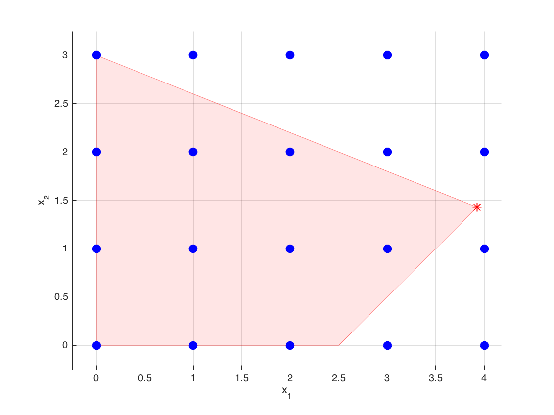
If you work out the details of the dictionary, you will see that the row corresponding to the basic variable $x_1$ reads
$$ x_1 + \frac{1}{7} x_3 + \frac{5}{14} x_4 = \frac{55}{14}, $$where $x_3$ and $x_4$ are the slack variables associated with the first and the second constraints, respectively. Then, the corresponding Gomory cut becomes
$$ \frac{1}{7} x_3 + \frac{5}{14} x_4 \geq \frac{13}{14} \iff \frac{1}{7} (15 - 2x_1 - 5x_2) + \frac{5}{14}(5 - 2x_1 + 2x_2) \geq \frac{13}{14} \iff x_1 \leq 3. $$Next, we add the cut and solve the resulting LP relaxation problem. Our implementation here does not take into account a possible warm-start due to adding only one row. Such a warm-start step with GLPK is not possible in GNU Octave. This could be achieved with a C++ or Java implementation. Please see the GLPK documentation.
A = [A; 1, 0];
b = [b; 3];
ctype = repmat("U", 1, 3);
[xopt, objval] = glpk(c, A, b, lb, ub, ctype, vartype, -1);
fprintf('\nOptimal objective function value: %f', objval);
fprintf('\nOptimal solution: '); xopt'
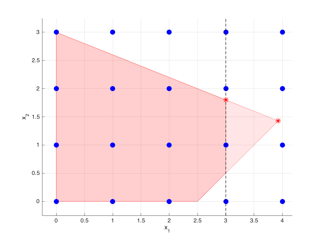
At the optimal dictionary, the row corresponding to the basic variable $x_2$ is given by
$$ x_2 + \frac{1}{5} x_3 - \frac{2}{5} x_5 = \frac{9}{5}, $$where $x_5$ is the slack variable associated with the most recently added constraint. Then, the corresponding Gomory cut becomes
$$ \frac{1}{5} x_3 + \frac{3}{5} x_5 \geq \frac{4}{5} \iff \frac{1}{5} (15 - 2x_1 - 5x_2) + \frac{3}{5}(3 - x_1) \geq \frac{4}{5} \iff x_1 + x_2 \leq 4. $$A new cut is ready to be added to our model.
A = [A; 1, 1];
b = [b; 4];
ctype = repmat("U", 1, 4);
[xopt, objval] = glpk(c, A, b, lb, ub, ctype, vartype, -1);
fprintf('\nOptimal objective function value: %f', objval);
fprintf('\nOptimal solution: '); disp(xopt')
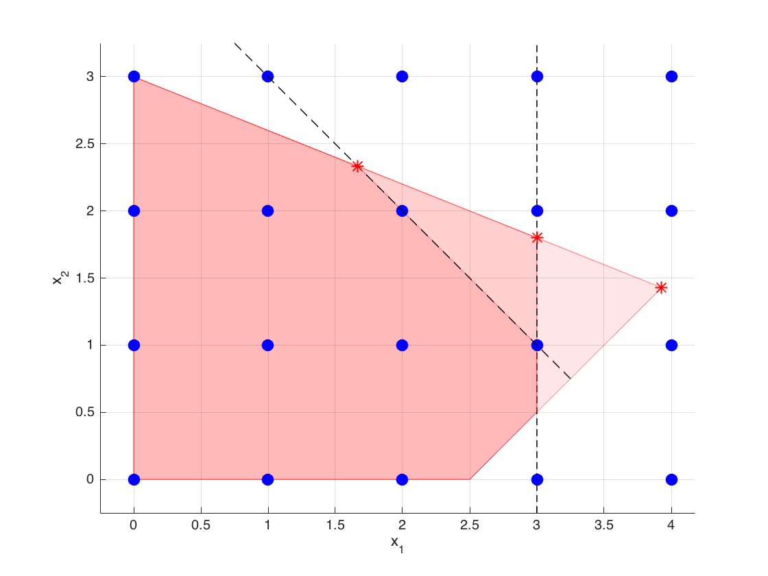
At the optimal dictionary, we again select the row corresponding to the basic variable $x_2$ given by
$$ x_2 + \frac{1}{3} x_3 - \frac{2}{3} x_6 = \frac{7}{3}, $$where $x_6$ is the slack variable associated with the most recently added constraint. Next, we can write down the new cut
$$ \frac{1}{3} x_3 + \frac{1}{3} x_6 \geq \frac{1}{3} \iff \frac{1}{3} (15 - 2x_1 - 5x_2) + \frac{1}{3}(4 - x_1 - x_2) \geq \frac{1}{3} \iff x_1 + 2x_2 \leq 6. $$Let's add the new cut to our model.
A = [A; 1, 2];
b = [b; 6];
ctype = repmat("U", 1, 5);
[xopt, objval] = glpk(c, A, b, lb, ub, ctype, vartype, -1);
fprintf('\nOptimal objective function value: %f', objval);
fprintf('\nOptimal solution: '); disp(xopt')
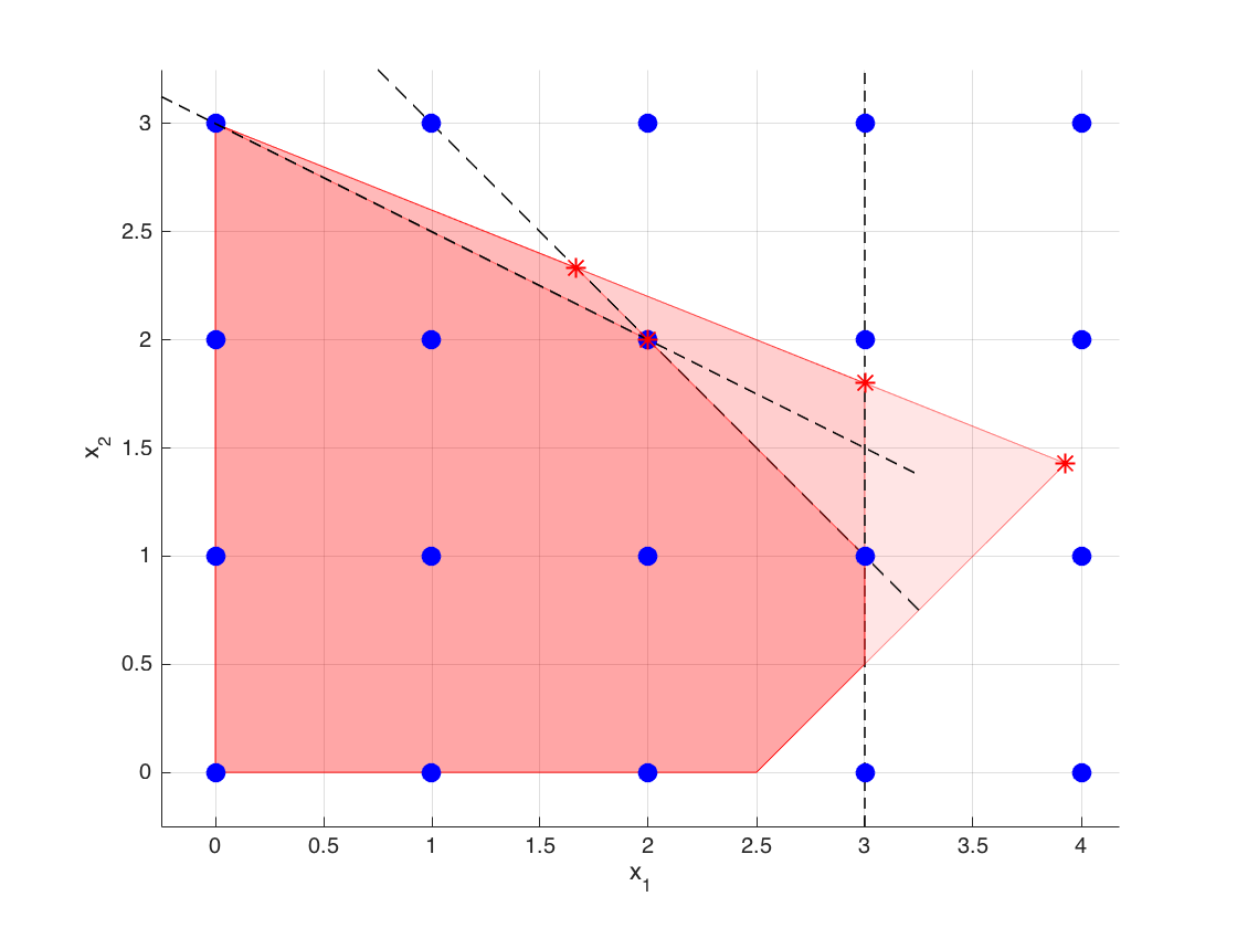
After the third cut we have found the optimal integer solution of our problem.
Our next section gives several cutting plane examples that are used for solving mixed integer programming (MIP) problems.
Mixed-Integer Rounding Inequalities
When we are dealing with MIP problems, Gomory cuts are not immediately applicable. Following the steps of Gomory, many people in the area of integer programming and combinatorial optimization have come up with different cut generation methods (Wolsey, 1999). Among these, a famous one is known as generation of mixed-integer rounding (MIR) inequalities. The notes here are mainly taken from the plenary talk of Oktay Günlük in 2010.
A fundamental MIR inequality follows after we define the following set
$$ \CS = \{x \in \RR, y \in \ZZ : x + y \geq b, x \geq 0\}. $$Then, it is not difficult to check that the MIR cut
$$ x + \hat{b} y \geq \hat{b}\lceil b \rceil, $$where $\hat{b}=(b - \lfloor b \rfloor)$, is valid for $\CS$ with
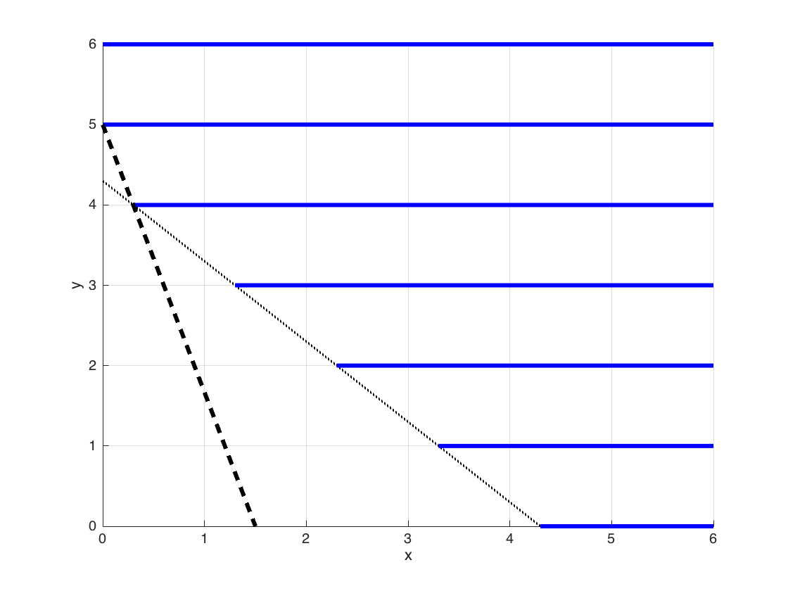
$$ conv(\CS) = \{x, y \in \RR : x + y \geq b, \ x + \hat{b} y \geq \hat{b}\lceil b \rceil, \ x \geq 0\}. $$We can illustrate this elementary cut with an example. Suppose we have
$$ \CS = \{x \in \RR, y \in \ZZ : x + y \geq 4.3, x \geq 0\}. $$Using the derivation above, we obtain
$$ conv(\CS) = \{x, y \in \RR : x + y \geq 4.3, \ x + 0.3y \geq 1.5, \ x\geq 0\}. $$In the figure below, the blue lines show the set $\CS$. Note that after adding the MIR inequality, the $y$ component of each extreme point becomes integral.
In fact, we can do better than dealing with only two variables. The derivation for a single constraint follows similar steps. Suppose our set is given as
$$ \CS = \{x \in \RR^{|\CU|}, y \in \ZZ^{|\CV|} : \sum_{j \in \CU} u_j x_j + \sum_{j \in \CV} v_j y_j \geq b, \ \ x, y \geq 0\}. $$Then, we rewrite this inequality
$$ \sum_{u_j < 0} u_j x_j + \sum_{u_j > 0} u_j x_j + \sum_{\hat{v}_j < \hat{b}} \hat{v}_j y_j + \sum_{\hat{v}_j \geq \hat{b}} \hat{v}_j y_j + \sum_{j \in \CV} \lfloor v_j \rfloor y_j \geq b = \hat{b} + \lfloor b \rfloor $$where $\hat{v}_j$ and $\hat{b}$ denote as before the fractional parts of $v_j$ and $b$, respectively. Next, we relax the constraint and obtain
$$ \underset{\geq 0}{\underbrace{\sum_{u_j > 0} u_j x_j + \sum_{\hat{v}_j < \hat{b}} \hat{v}_j y_j}} + \underset{\in \ZZ}{\underbrace{\sum_{\hat{v}_j \geq \hat{b}} y_j + \sum_{j \in \CV} \lfloor v_j \rfloor y_j}} \geq b. $$This allows us to use the elementray MIR cut above
$$ \sum_{u_j > 0} u_j x_j + \sum_{\hat{v}_j < \hat{b}} \hat{v}_j y_j + \hat{b}\left(\sum_{\hat{v}_j \geq \hat{b}} y_j + \sum_{j \in \CV} \lfloor v_j \rfloor y_j\right) \geq \hat{b}\lceil b \rceil. $$Of course, the natural next step is to consider a group of constraints. In this case our set becomes $$ \CS = \{x \in \RR^{|\CU|}, y \in \ZZ^{|\CV|} : Ux + Vy \geq d, \ \ x, y \geq 0\}. $$
where $U$ is an $m \times |\CU|$ and $V$ is an $m \times |\CV|$ matrices.
Let $\lambda \geq 0$ be an $m$-dimensional row vector. Clearly,
$$ \lambda Ux + \lambda Vy \geq \lambda d. $$Then, we can write the MIR cut
$$ \sum_{j \in \CU} \max\{0, \lambda U_j\}x_j + \hat{b} \sum_{j \in V} \lfloor \lambda V_j\rfloor y_j + \sum_{j \in \CV} \min\{ \lambda V_j - \lfloor \lambda V_j\rfloor, \hat{b}\}y_j \geq \hat{b}\lceil \lambda d\rceil, $$where $\hat{b} = \lambda d - \lceil \lambda d\rceil$ along with $U_j$ and $V_j$ denoting the $j$th column of $U$ and $V$, respectively.
We can wrap up this section with one last example. Suppose the feasible set is given by
$$ \CS = \{x \in \RR, y \in \ZZ : -x-4y \geq -4, \ -x+4y \geq 0, \ x,y \geq 0\}. $$For any $\lambda_1, \lambda_2 \geq 0$, we have
$$ (-\lambda_1 - \lambda_2) x + (-4 \lambda_1 + 4\lambda_2)y \geq -4\lambda_1. $$Clearly, the coefficient of $x$ is always negative. Thus, we focus on the inequality
$$ (-4 \lambda_1 + 4\lambda_2)y \geq -4\lambda_1 $$Let now $\lambda_1 = \frac{1}{8}$ and $\lambda_2=\frac{1}{4}$. Then
$$ -\frac{1}{2}y + y \geq -\frac{1}{2} \implies \frac{1}{2}y \geq -\frac{1}{2} $$with $\hat{b} = -\frac{1}{2}-\lceil -\frac{1}{2}\rceil = -\frac{1}{2}$. This leads to the MIR cut
$$ \min\left\{-\frac{1}{2}-(-1), -\frac{1}{2}\right\}y \geq (-\frac{1}{2})0 \implies y \leq 0, $$which is a pretty strong cut.
Concluding Remarks
We have barely scratched the surface of the vast subject of cutting plane methods. There are many other general cuts; such as, lattice-free cuts, crooked crossed cuts, split cuts, odd-cycle inequalities, cover inequalities, lift-and-project cuts and so on. These are beyond the scope of this class.
Our dicussion in this lecture is based on (mixed) integer programming problems. However, the cutting plane methods are also used in nonlinear programming, in particular, for convex optimization on a polyhedron (Kelley, 1960).
Papers for Next Week's Discussion
- Gomory, R. E. (1958). Outline of an algorithm for integer solutions to linear programs, Bull. Amer. Math. Soc. 64:5, 275-278.
- Kelley, J. E. Jr. (1960). The cutting-plane method for solving convex programs, J. Soc. Indust. Appl. Math., 8:4, 703-712.
- Guan, Y., Ahmed, S. and G. L. Nemhauser (2009). Cutting planes for multistage stochastic integer programs, Operations Research, 57:2, 287-298.
References
- Gomory, R. E. (1958). Outline for an algorithm for integer solutions to linear programs, Bulletin of the American Mathematical Society, 64, 275-278.
- Wiesemann, W. (2009). Integer programming lecture notes, website - Last accessed 22 February 2016.
- Wolsey, L. A. and G. L. Nemhauser (1999). Integer and Combinatorial Optimization, Wiley Series in Discrete Mathematics and Optimization (Book 15), A Wiley-interscience publication.
- Günlük, O. (2010). Cutting planes for mixed-integer programs, Plenary talk at the 30th National Congress on Operations Research and Industrial Engineering, July 2010, Istanbul.
- Kelley, J. E. Jr. (1960). The cutting plane method for solving convex programs, J. Soc. Indust. Appl. Math., 8:4, 703-712.